Lesson 9: Clustering¶

Syntax note:

Note that in Python syntax, you will have to use a dot to specify where you want to get a function from. For example, there is a package called numpy, with a module called random, with a function called seed. The seed function is called by typing out np.random.seed(), telling python where exactly it needs to look.

WE ARE USING PYTHON3, NOT PYTHON

General Factoids¶

Clustering: The process of partitioning a dataset into groups based on shared unkown characteristics. In other words, we are looking for patterns in data where we do not necessarily know the patterns to look for ahead of time.

In: N points, usually in the form of a matrix(each row is a point).

In: A distance function to tell us how similar two points are. The most intuitive distance function is euclidean distance. The type of distance measure you use can vary depending on the type of data you are using. One specific example of how fine tuned distance metrics can be is a distance metric that weights substitutions in DNA strings heavier than indels because indels are more common sequencing errors. This means that such a metric would not separate two DNA strands due to sequencing error.

Out: K groups, each containing points which are similar to each other in some way. Some algorithms cluster for a preset number K, others figure it out as they go along.

How is DNA a point? One common way we translate DNA strings to points is by making a string of DNA into a kmer vector. A kmer is a string of length k, and there are 4^k possible kmers in any DNA strand. Usually we think of kmers as ordered lexicographically like this: AAA, AAC, AAG, AAT, ACA, ACC, ACG, ACT, AGA and so on. One way to represent a DNA strand is to create an array of zeros of length 4^k and increment by one for each time that kmer appears in the DNA strand.

Problem: Find the kmer vector of “AG” (k=2).

Bioinformatics Applications of Clustering:¶

Finding what genes are up and down regulated under certain conditions. Imagine you have a matrix, where each point is a set of gene expression recorded for a variety of conditions. If two points are close to each other, that means they had similar expression levels throughout those conditions.
Discerning different species present in a sample of unkown contents. This can be done with an algorithm that does not have a predetermined amount of clusters. An example application is taking HIV sequences from a patient, clustering them, and filtering clusters under a certain size to find the sequences of prevalent strains within the patient.
Finding evolutionary relationships between samples using hierarchical clustering. The earlier on two centers were combined, the closer their corresponding points are from an evolutionary perspective.

Generating Data¶

In order to demonstrate the differences between different clustering methods, we need datasets that cluster differently depending on technique.

Copy the starter file into your directory:

https://drive.google.com/file/d/13j7v4lUOfWY4PhR9mT1-SBao8FkitbEh/view?usp=sharing

This file clust.py contains a plotting function - don’t touch it! We will be creating stuff for that plotting function to plot in a minute, so write your code below that function.

Start by creating some blobs using numpy’s random normal generator. First, create a seed for the random number generator with

np.random.seed()

Make a few blobs of points (probably two) with centers between 0 and 20 and varied stdevs (keeping the array dimensions the same). Example syntax: clust1 = np.random.normal(5, 2, (1000,2))

Put the point blobs into one structure so that we can cluster them all at once with

dataset1 = np.concatenate()

We will be comparing how our point blobs cluster to the way that circles of datapoints cluster. Create two concentric circles as the second dataset. dataset2 = datasets.make_circles(n_samples=1000, factor=.5, noise=.05)[0]

If you want to see what your datasets look like, use the cluster_plots function

Note: cluster_plots will save your plots to a pdf file in your current directory, the name of which can be changed.

scp username@ec2-3-135-188-28.us-east-2.compute.amazonaws.com:/home/username/path /localpath/

Clustering Data¶

1. K-means¶

Steps:¶

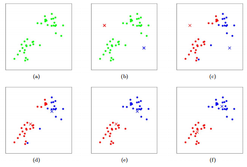
(We present the Lloyd Algorithm here, but there are other algorithms for k-means clustering) I. Select K centers. This can be done a variety of ways, the easiest of which is to select k random points; maybe find a random point, find the farthest point from that and select it, find the furthest point from the previous and so on; this is called farthest first traversal

II. Assign each point to the center nearest to it. (Centers to Clusters step)

III. For each center, take all the points attached to it and take their average to create a new center for that cluster.

IV. Reassign all points to their nearest center (Clusters to Centers step) and continue reassigning + averaging until the iteration when nothing changes.

Code:¶

We will be using the KMeans algorithm from sklearn’s cluster package to dataset1 and dataset2. Remember that k is the number of clusters the KMeans algorithm will assign points to, so give Kmeans the appropriate k. The points returned from the KMeans function will be separated into clusters, making them easy for the cluster_plots function to distinguish and color accordingly.

kmeans_dataset1 = cluster.KMeans(n_clusters=k).fit_predict(dataset1)
cluster_plots(dataset1, dataset2, kmeans_dataset1, kmeans_dataset2)

(While using the sklearn implementation as a black box is the general practice as we’ve seen so far, it is a good learning practice and a nice coding challenge to implement the Lloyd Algortihm yourself. Check out this Rosalind problem “Implement the Lloyd Algorithm for k-Means Clustering” (You could solve the previous problem on Rosalind for distance calculation)

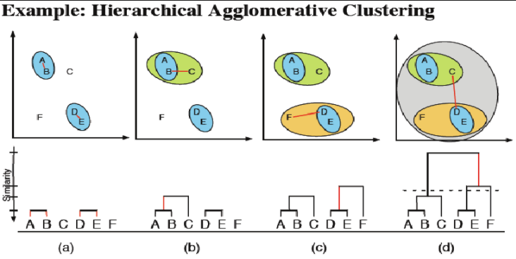
2. Agglomerative Hierarchical¶

Description:¶

I. Start with every point being its very own cluster center.

II. Find the two centers which are closest to each other and combine them into one cluster. The new center is the average of the two previous ones.

III. Continue combining the closest centers until all points are under a single cluster.

Code:¶

Let’s look at the blobs and circles we made again. Look at the documentation page for agglomerative clustering and figure out the proper calls for the two datasets (syntax is very similar to what you did for k-means).

Now, run cluster_plots() to graph and scp to view the results. Do you notice a difference in quality of the clustering of the left and right graphs?

Unfortunately, this still does not solve our circlular cluster issue. For that, we can ask the sklearn package to build a graph out of our circles which restricts the amount of nearest neighbors a point can cluster with.

#this line limits the number of nearest neighbors to 6
connect = kneighbors_graph(dataset2, include_self=False, n_neighbors = 6)

#in this line, you need to set linkage to complete, number of clusters to 2, and set connectivity equal to the graph 
#on the previous line
hc_dataset2_connectivity = cluster.AgglomerativeClustering().fit_predict(dataset2)

Use cluster_plots() to graph the plot resulting from the regular AgglomerativeClustering beside the graph that plots the connected AgglomerativeClustering. As you may have guessed, this fixes the circle problem.

3. Soft Clustering¶

Description:¶

This is essentially the same thing as k-means, but points cannot be hard assigned to a cluster. Instead, each point has a probability of being in each cluster, and points with higher probabilities influence the center of that cluster more.

I. Select K centers randomly (or slightly less randomly, like farthest first traversal.

II. Expectation step: Assign a responsibility (a likelihood) for each point in respect to each cluster. Basically, the closer a point is to a center the higher the likelyhood of that point. This can be calculated in a variety of ways, but the main idea is that it is some function relating the distance from a point to a center to the distances between all points and that center to see if it is much closer or further than other points

III. Maximization step: compute new cluster centers by using a weighted average of the points based on the likelihoods calculated in step II.

Code:¶

Let’s go ahead and see what will happen with our blobs and circles under this clustering algorithm:

em_set1=mixture.GaussianMixture().fit_predict()

Use these new clusters in our cluster_plots()

Also feel freee to check out Rosalind problem “Implement the Soft k-Means Clustering Algorithm”](http://rosalind.info/problems/ba8d/).

Challenge¶

Head over here to complete our clustering challenge!

Credits¶

Lloyd Algorithm k-means clustering and Soft Clustering explanation and challenge are adapted from Rosalind, particularly Rosalind problem “Implement the Lloyd Algorithm for k-Means Clustering” and Rosalind problem “Implement the Soft k-Means Clustering Algorithm”