Lesson 11: Phylogenetics
The Basics
What is Phylogenetics?
At its core, phylogenetics is the study of finding evolutionary relationships between organisms. How, you ask? By looking for similarities (in our case, on the DNA level). Let’s pose one such problem:
Imagine you’re given five distinct organisms and are told to figure out how they’re evolutionarily related (that is, how they evolved from one another). Two questions pop into your head: Why? and How?
Why Do I Care?
The answer is twofold:
- On a broader scale, an understanding of phylogenetics gives us a better understanding of the living world, and how we + our fellow organisms fall into it. We can answer questions about how we are linked to jellyfish, and how that relationship has shaped the world around us.
- On a smaller scale, phylogenetics also provides key information about genetic drift, the evolution of genes and diseases, and the development of molecular differences between organisms.
How Does it Work?
We need some shared, conserved mechanism of comparing the organisms… something like DNA! There are sequences in DNA that are highly conserved between organisms (usually sequences that code for absolutely essential parts of life) that are excellent candidates for comparison. For example, imagine you have three organisms with the following sequence of DNA in a conserved region:
1. ACGTG
2. ACGTC
3. ACGCC
We can compare the nucleotides at each position and find that 1 and 2 differ by one nucleotide, 2 and 3 differ by one nucleotide, but 1 and 3 differ by two nucleotides. This might lead you to conclude that the relationship between organisms 1 and 3 is the most evolutionarily distant.
Note: In reality, these conserved sequences are much, much longer, and the analysis is far more robust than counting of a few nucleotides.
Biopython
If you’re not familiar with Biopython, please skim our previous lesson here.
If you know what you’re doing, running this on your own machine instead of on EC2 will probably give you some nicer graphs. This is optional, continue on EC2 if you wish!
You’ll need to have Biopython installed to continue (done for you on EC2). Confirm by running a Python program with the following:
from Bio import Phylo
If nothing shows up during execution, you’re good to go!
Find the Relationships
Working with Trees
 phylo_tree
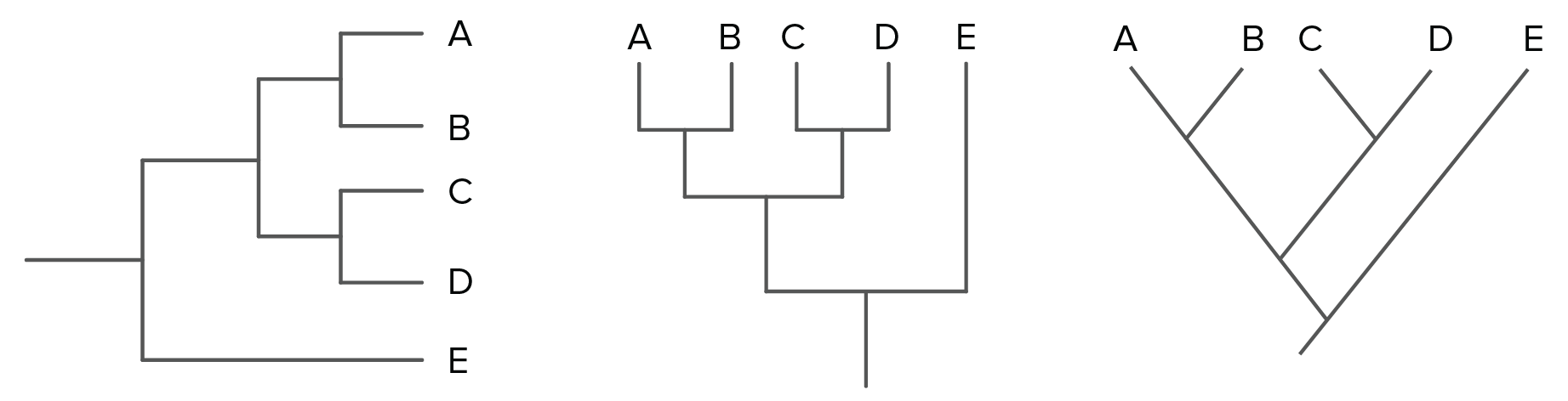
You’ve probably seen one or more of the phylogenetic trees diagrammed above. These visually represent the heart and soul of phylogenetics. Because we use a last universal common ancestor model (LUCA model), in which the root represents an ancestral organism from which all living organisms today evolved, each evolutionary relationship can be represented by a branching of the tree.
The Data
Let’s see this in action with our own phylogenetic tree! Remember those five organisms we mentioned earlier? Well here they are, each with a conserved DNA region sequenced:
   5   13
Alpha     AACGTGGCCACAT
Beta      AAGGTCGCCACAC
Gamma     CAGTTCGCCACAA
Delta     GAGATTTCCGCCT
Epsilon   GAGATCTCCGCCC
Note: The first line is a header. The first number is the number of organisms, and the second is the length of each DNA sequence.
Copy and paste all of the data above (including the header file) into a new file called msa.phy. The .phy extension indicates that the file contains phylogenetic data.
What kind of data goes into making trees?
As with basically all other programs dealing with biological sequences, phylogenetics algorithms need you to align your sequences before you input them, so that they are easier to compare. If you are curious about different methods of alignment and their influence on the final alignment go over to our lesson on alignment over here.
The Setup
Now we’re ready to start analyzing this data. Create a new python file and add the following to import everything we need:
from Bio import Phylo
from Bio.Phylo.TreeConstruction import DistanceCalculator
from Bio.Phylo.TreeConstruction import DistanceTreeConstructor
from Bio import AlignIO
Make sure you can run this file without errors!
Here’s some documentation that may help you if you get stuck: AlignIO, DistanceCalculator, DistanceTreeConstructor
Note: If you’re not able to follow the instructions below, ask the bootcamp developers for a templated file to help guide you!
Alignment
The first step is to import the (already aligned) sequences into our program. Use AlignIO to read in the data, and store it in a variable aln. Print aln to confirm this step worked correctly.
Distance Matrix
Now that we have our data, we’re interested in how similar (or different) the sequences are from each other. The more similar, the more likely they are to be evolutionarily close. Therefore, we use a distance matrix to store information on how similar each DNA sequence is from every other sequence. Create a Distance Calculator object with the ‘identity’ model. Use it to calculate the distance matrix of the alignment, and store it in a variable dm.
Phylogenetic Tree
Now, the real magic… creating the phylogenetic tree! We can use our Distance Tree Constructor to make a tree from our distance matrix. Use the UPGMA algorithm in Distance Tree Constructor to create a tree and store it in a variable tree.
Visualization
Great, you’re done! Except… you’re probably interested in how your tree turned out! The simplest way to visualize your tree is to use the Phylo.draw_ascii() method to print the tree to the terminal. This will give you a low-detail sketch of your tree. Make sure you can do this before moving forward.
You’re probably interested in a much more detailed tree, though. The Phylo.draw() method provides that, but requires matplotlib as a dependency (pip install matplotlib if you don’t have it [EC2 does!]).
Interpretation
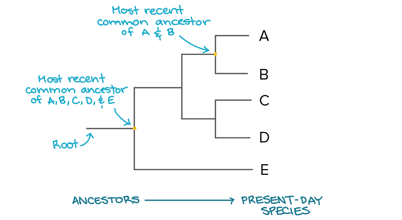
Phylogenetic trees are interpreted using the following terms:
 tree
tree
How many common ancestors are there? What does that tell you about the relationships and evolutionary distances between the organisms.
Challenge: Different Algorithms, Different Results
We made two algorithm choices in our pipeline above. One is the distance calculator’s model and the other is the distance tree’s model. Use the documentation to find alternate algorithms and try various combinations. You’ll see the predicted tree (and the evolutionary relationships) change!
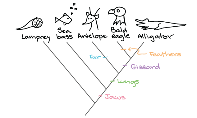
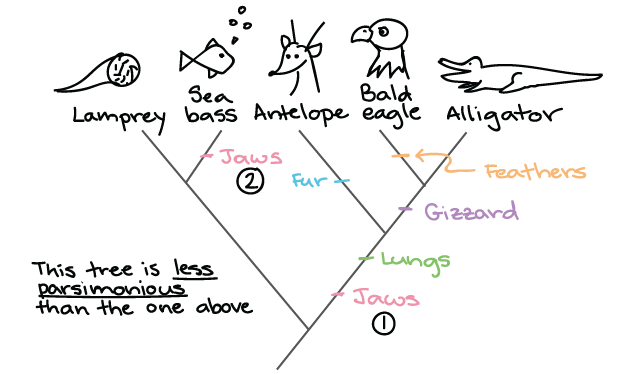
How do we know which tree is the best? Let’s look at an analogous example with phenotypic mutations that’s easier to follow than genotypic mutations. Consider the two trees below:
 tree1
tree1
 tree2
tree2
The first tree is a better prediction because it relies on less evolutionary events to happen independent of each other (less “parsimony”). Think: If you and your roommate are both sitting on the couch eating stawberry popsicles with chia seeds, it’s more likely that the popsicles came from the same source than two independent sources.
Looking at the different trees the algorithms produced, do you have a favorite? (There’s no real right answer here… we don’t know how these sequences evolved! As long as your can justify your choice, you’re good.)
So, what are these models we’re switching between? Let’s take a look:
Distance Tree Models
Unweighted Pair-Group Method with Arithmetic Averaging (UPGMA)
This model is heavily based upon the assumption that there is an equal rate of evolution (resulting in all branch lengths being the same in the tree). This is a VERY POOR assumption, which makes this model rather unreliable.
Distance Calculation Methods
Identity
Distance is equal to the proportion of non matching nucleotides, so lower distance = closer relationship.
Blastn
Matches are worth 5 points, while mismatches are worth -4 points. The formula to calculate the final score is:
1 - (matches*5-mismatches\*4)/(length\*5).
Trans
This scoring takes the difference in transitions(purine->purine or pyrimidine->purine) vs transversions(purine->pyrimidine and vice versa) into account. Transversions are less likely to occur, so they are scored -6 compared to the -1 for transitions. Matches are given a score of 6.
Acknowledgements
Many data and algorithms are adapted from the offical Biopython textbook.Algorithm adapted from Towards Data Science. Diagrams adapted from Khan Academy.